Plotting maps with sp
This document shows example images created with objects represented by one of the classes for spatial data in packages sp.
Loading data and packages
The Meuse data set is loaded using a demo script in package
sp,
## [1] "SpatialPointsDataFrame"
## attr(,"package")
## [1] "sp"
The North Carolina SIDS (sudden infant death syndrome) data set is
available from package sf, and is loaded by
## Linking to GEOS 3.10.2, GDAL 3.4.1, PROJ 8.2.1; sf_use_s2() is TRUE
nc <- as(st_read(system.file("gpkg/nc.gpkg", package="sf")), "Spatial")## Reading layer `nc.gpkg' from data source
## `/home/runner/work/_temp/Library/sf/gpkg/nc.gpkg' using driver `GPKG'
## Simple feature collection with 100 features and 14 fields
## Geometry type: MULTIPOLYGON
## Dimension: XY
## Bounding box: xmin: -84.32385 ymin: 33.88199 xmax: -75.45698 ymax: 36.58965
## Geodetic CRS: NAD27Using base plot
The basic plot command on a Spatial object
gives just the geometry, without axes:
plot(meuse)
axes can be added when axes=TRUE is given; plot elements
can be added incrementally:
plot(meuse, pch = 1, cex = sqrt(meuse$zinc)/12, axes = TRUE)
v = c(100,200,400,800,1600)
legend("topleft", legend = v, pch = 1, pt.cex = sqrt(v)/12)
plot(meuse.riv, add = TRUE, col = grey(.9, alpha = .5))
For local projection systems, such as in this case
proj4string(meuse)## [1] "+proj=sterea +lat_0=52.1561605555556 +lon_0=5.38763888888889 +k=0.9999079 +x_0=155000 +y_0=463000 +ellps=bessel +units=m +no_defs"the aspect ratio is set to 1, to make sure that one unit north equals one unit east. Even if the data are in long/lat degrees, an aspect ratio is chosen such that in the middle of the plot one unit north approximates one unit east. For small regions, this works pretty well; also note the degree symbols in the axes tic marks:
crs.longlat = CRS("+init=epsg:4326")## Warning in CPL_crs_from_input(x): GDAL Message 1: +init=epsg:XXXX syntax is
## deprecated. It might return a CRS with a non-EPSG compliant axis order.
meuse.longlat = spTransform(meuse, crs.longlat)
plot(meuse.longlat, axes = TRUE)
which looks different from the plot where one degree north (latitude) equals one degree east (longitude):

Graticules
Instead of axes with ticks and tick marks, maps often have
graticules, a grid with constant longitude and latitude lines.
sp provides several helper functions to add graticules,
either in the local reference system, or in long/lat. Here is an example
of the local reference system:
par(mar = c(0, 0, 1, 0))
library(methods) # as
plot(as(meuse, "Spatial"), expandBB = c(.05, 0, 0, 0))
plot(gridlines(meuse), add = TRUE, col = grey(.8))
plot(meuse, add = TRUE)
text(labels(gridlines(meuse)), col = grey(.7))
title("default gridlines with Meuse projected data")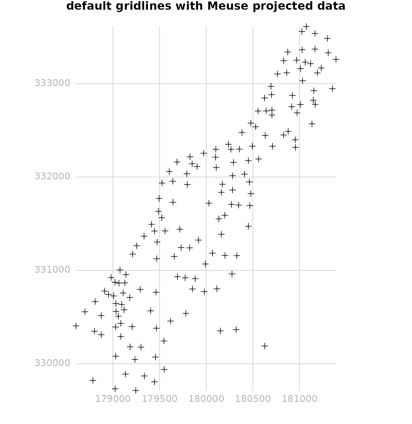
par(mar = c(0, 0, 1, 0))
grd <- gridlines(meuse.longlat)
grd_x <- spTransform(grd, CRS(proj4string(meuse)))
plot(as(meuse, "Spatial"), expandBB = c(.05, 0, 0, 0))
plot(grd_x, add=TRUE, col = grey(.8))
plot(meuse, add = TRUE)
text(labels(grd_x, crs.longlat), col = grey(.7))
## Warning in labels.SpatialLines(grd_x, crs.longlat): this labels method is meant
## to operate on SpatialLines created with sp::gridlines
title("longitude latitude gridlines and labels")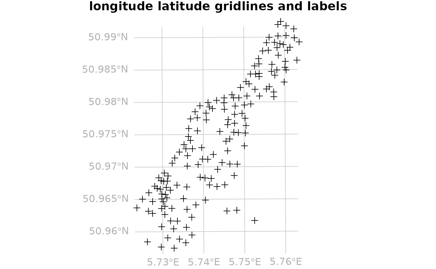
These lines look pretty straight, because it concerns a small area. For
# demonstrate axis labels with angle, both sides:

maps2sp = function(xlim, ylim, l.out = 100, clip = TRUE) {
    stopifnot(require(maps))
    m = map(xlim = xlim, ylim = ylim, plot = FALSE, fill = TRUE)
    as(st_as_sf(m), "Spatial")
}
par(mar = c(0, 0, 1, 0))
m = maps2sp(c(-100,-20), c(10,55))
## Loading required package: maps
sp = SpatialPoints(rbind(c(-101,9), c(-101,55), c(-19,9), c(-19,55)), CRS("+init=epsg:4326"))
laea = CRS("+proj=laea +lat_0=30 +lon_0=-40")
m.laea = spTransform(m, laea)
sp.laea = spTransform(sp, laea)
plot(as(m.laea, "Spatial"), expandBB = c(.1, 0.05, .1, .1))
plot(m.laea, col = grey(.8), add = TRUE)
gl = gridlines(sp, easts = c(-100,-80,-60,-40,-20), norths = c(20,30,40,50))
gl.laea = spTransform(gl, laea)
plot(gl.laea, add = TRUE)
text(labels(gl.laea, crs.longlat))
## Warning in labels.SpatialLines(gl.laea, crs.longlat): this labels method is
## meant to operate on SpatialLines created with sp::gridlines## Warning in labels.SpatialLines(gl.laea, crs.longlat, side = 3:4): this labels
## method is meant to operate on SpatialLines created with sp::gridlines
title("curved text label demo")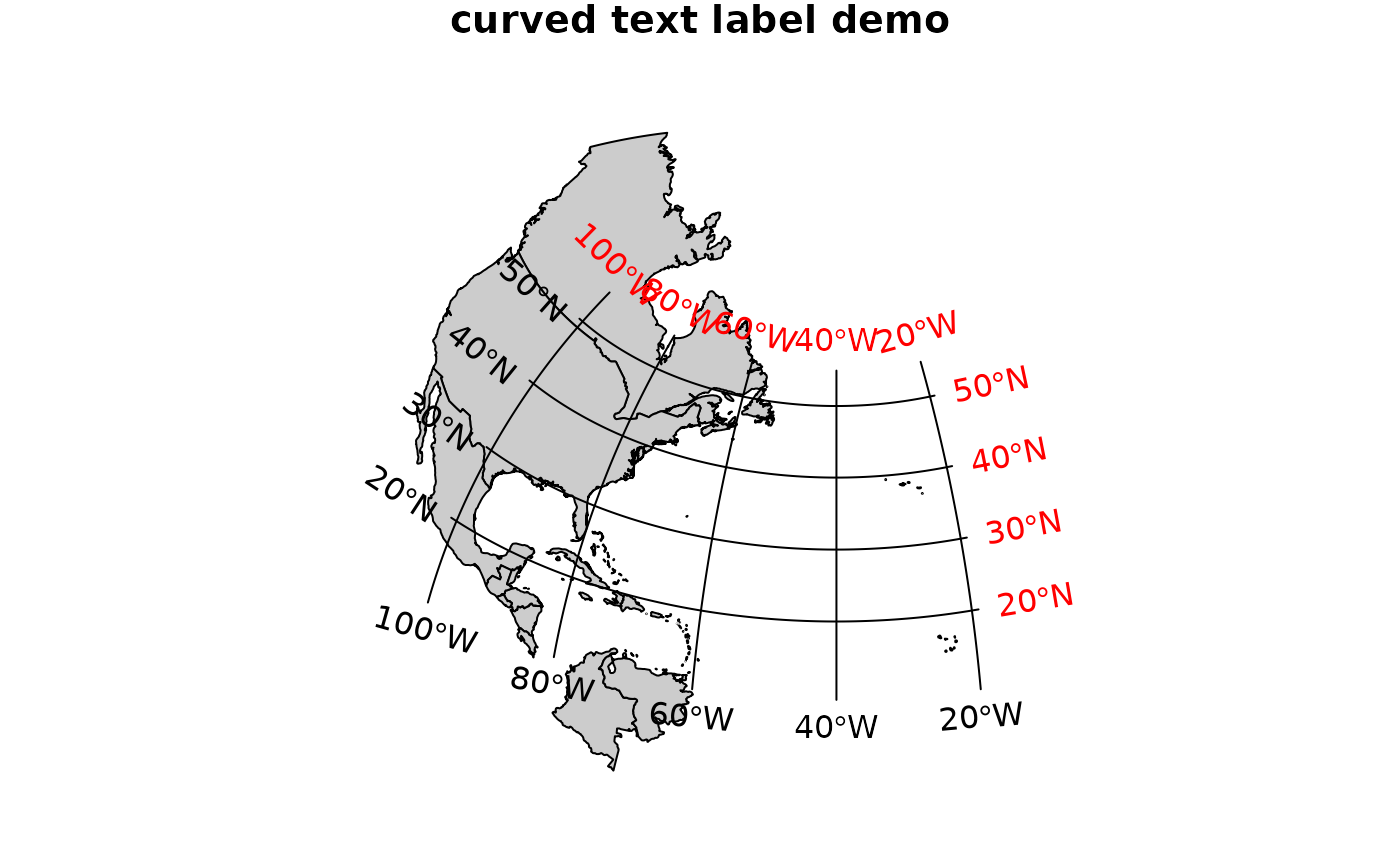
# polar:
par(mar = c(0, 0, 1, 0))
pts=SpatialPoints(rbind(c(-180,-70),c(0,-70),c(180,-89),c(180,-70)), CRS("+init=epsg:4326"))
gl = gridlines(pts, easts = seq(-180,180,20), ndiscr = 100)
polar = CRS("+init=epsg:3031")
plot(spTransform(pts, polar), expandBB = c(.05, 0, .05, 0))
gl.polar = spTransform(gl, polar)
lines(gl.polar)
l = labels(gl.polar, crs.longlat, side = 3)
## Warning in labels.SpatialLines(gl.polar, crs.longlat, side = 3): this labels
## method is meant to operate on SpatialLines created with sp::gridlines
l$pos = NULL # pos is too simple, use adj:
text(l, adj = c(0.5, -0.5), cex = .8)
l = labels(gl.polar, crs.longlat, side = 4)
## Warning in labels.SpatialLines(gl.polar, crs.longlat, side = 4): this labels
## method is meant to operate on SpatialLines created with sp::gridlines
l$srt = 0 # otherwise they end up upside-down
text(l, cex = .8)
title("grid line labels on polar projection, epsg 3031")
par(mar = c(0, 0, 1, 0))
m = maps2sp(xlim = c(-180,180), ylim = c(-90,-70), clip = FALSE)
gl = gridlines(m, easts = seq(-180,180,20))
polar = CRS("+init=epsg:3031")
gl.polar = spTransform(gl, polar)
plot(as(gl.polar, "Spatial"), expandBB = c(.05, 0, .05, 0))
plot(gl.polar, add = TRUE)
plot(spTransform(m, polar), add = TRUE, col = grey(0.8, 0.8))
l = labels(gl.polar, crs.longlat, side = 3)
## Warning in labels.SpatialLines(gl.polar, crs.longlat, side = 3): this labels
## method is meant to operate on SpatialLines created with sp::gridlines
# pos is too simple here, use adj:
l$pos = NULL
text(l, adj = c(0.5, -0.3), cex = .8)
l = labels(gl.polar, crs.longlat, side = 2)
## Warning in labels.SpatialLines(gl.polar, crs.longlat, side = 2): this labels
## method is meant to operate on SpatialLines created with sp::gridlines
l$srt = 0 # otherwise they are upside-down
text(l, cex = .8)
title("grid line labels on polar projection, epsg 3031")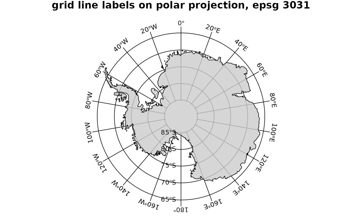
Other spatial objects in base plot
The following plot shows polygons with county name as labels at their center point:
par(mar = c(0, 0, 1, 0))
plot(nc)
invisible(text(coordinates(nc), labels=as.character(nc$NAME), cex=0.4))
This plot of a SpatialPolygonsDataFrame uses grey
shades:
names(nc)## [1] "AREA" "PERIMETER" "CNTY_" "CNTY_ID" "NAME" "FIPS"
## [7] "FIPSNO" "CRESS_ID" "BIR74" "SID74" "NWBIR74" "BIR79"
## [13] "SID79" "NWBIR79"
rrt <- nc$SID74/nc$BIR74
brks <- quantile(rrt, seq(0,1,1/7))
cols <- grey((length(brks):2)/length(brks))
dens <- (2:length(brks))*3
par(mar = c(0, 0, 1, 0))
plot(nc, col=cols[findInterval(rrt, brks, all.inside=TRUE)])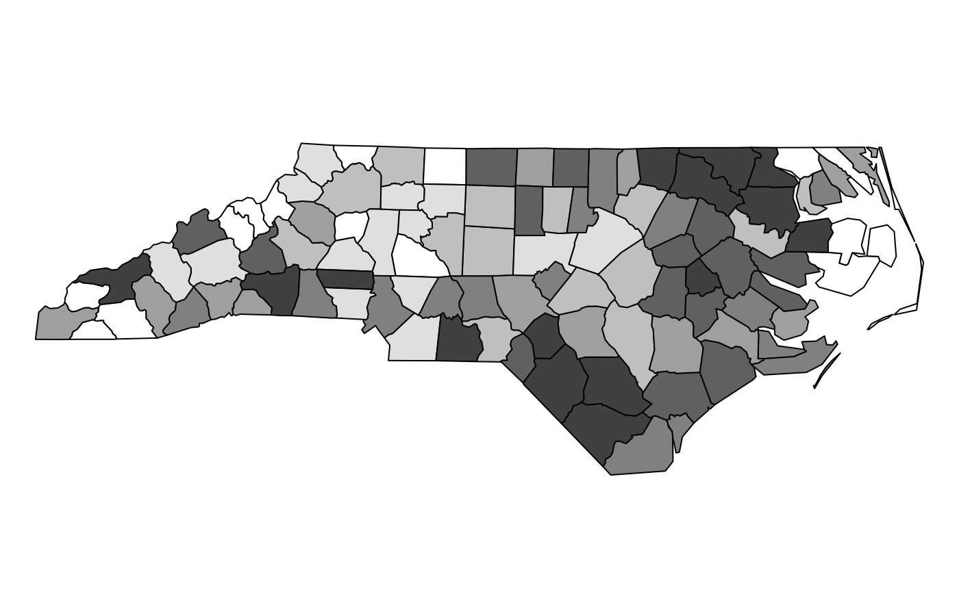
The following plot shows a SpatialPolygonsDataFrame,
using line densities
rrt <- nc$SID74/nc$BIR74
brks <- quantile(rrt, seq(0,1,1/7))
cols <- grey((length(brks):2)/length(brks))
dens <- (2:length(brks))*3
par(mar = rep(0,4))
plot(nc, density=dens[findInterval(rrt, brks, all.inside=TRUE)])
Plot/image of a grid file, using base plot methods:
image(meuse.grid)
Read this blog post to find out more about the options available (and limitations) for plotting gridded data with base plot methods in sp.
using lattice plot (spplot)
The following plot colours points with a legend in the plotting area and adds scales:
spplot(meuse, "zinc", do.log = TRUE,
    key.space=list(x = 0.1, y = 0.95, corner = c(0, 1)),
    scales=list(draw = TRUE))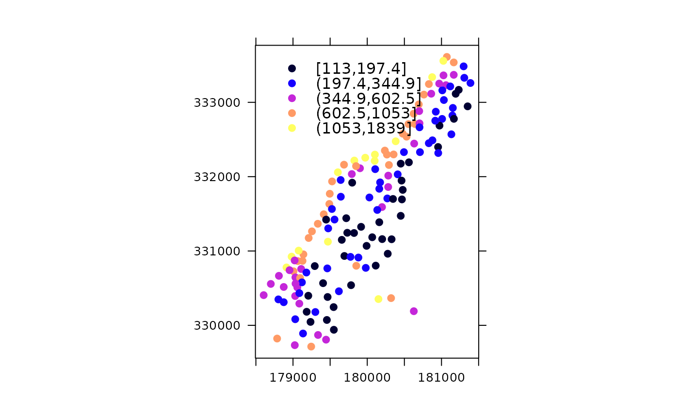
The following plot has coloured points plot with legend in plotting area and scales; it has a non-default number of cuts with user-supplied legend entries:
spplot(meuse, "zinc", do.log = TRUE,
    key.space=list(x=0.2,y=0.9,corner=c(0,1)),
    scales=list(draw = TRUE), cuts = 3,
    legendEntries = c("low", "intermediate", "high"))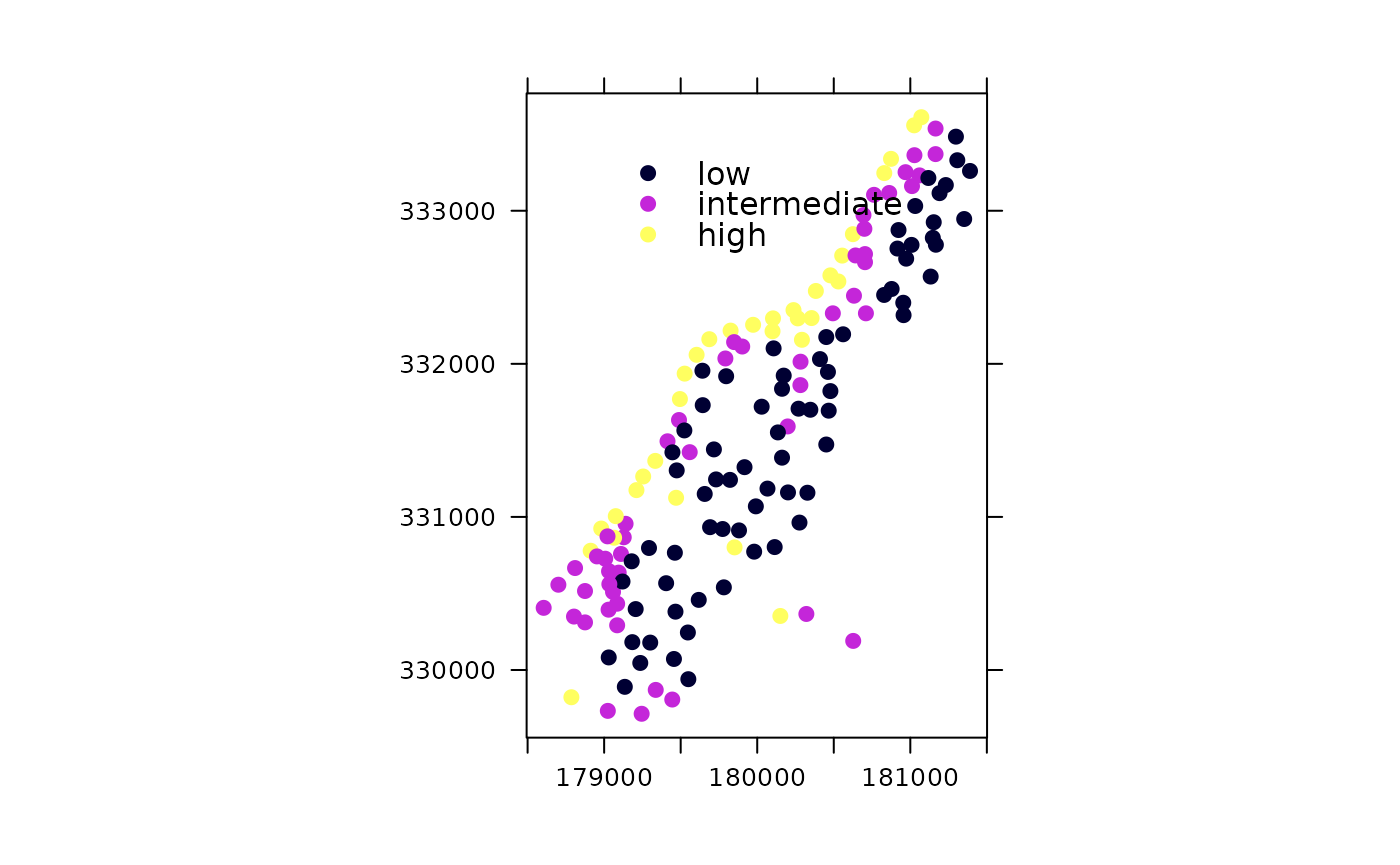
The following plot adds a scale bar and north arrow:
scale = list("SpatialPolygonsRescale", layout.scale.bar(),
    offset = c(178600,332490), scale = 500, fill=c("transparent","black"))
text1 = list("sp.text", c(178600,332590), "0")
text2 = list("sp.text", c(179100,332590), "500 m")
arrow = list("SpatialPolygonsRescale", layout.north.arrow(),
    offset = c(178750,332000), scale = 400)
spplot(meuse, "zinc", do.log=T,
    key.space=list(x=0.1,y=0.93,corner=c(0,1)),
    sp.layout=list(scale,text1,text2,arrow),
    main = "Zinc (top soil)")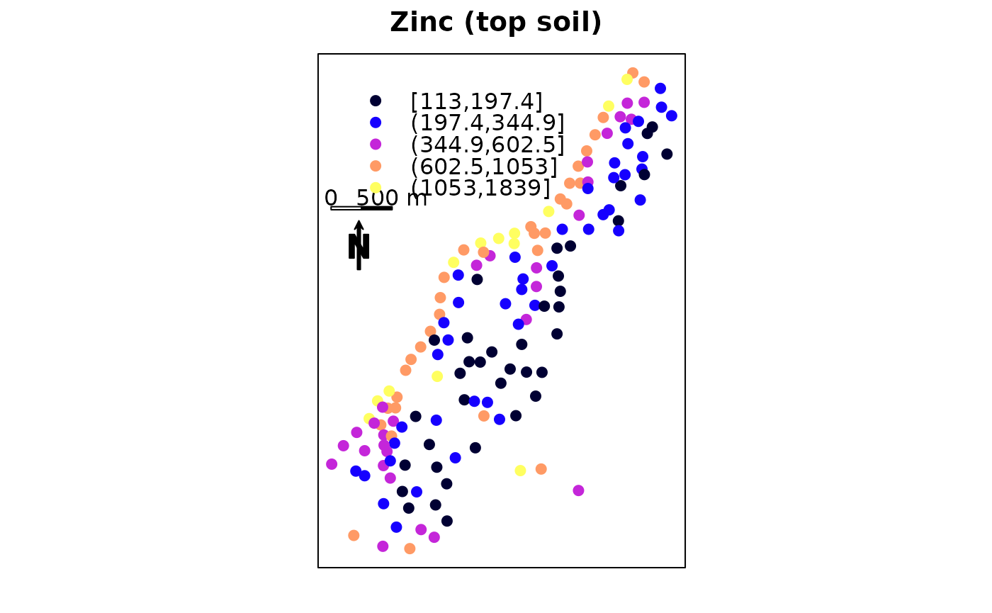
The following plot has north arrow and text outside panels
rv = list("sp.polygons", meuse.riv, fill = "lightblue")
scale = list("SpatialPolygonsRescale", layout.scale.bar(),
    offset = c(180500,329800), scale = 500, fill=c("transparent","black"), which = 1)
text1 = list("sp.text", c(180500,329900), "0", which = 1)
text2 = list("sp.text", c(181000,329900), "500 m", which = 1)
arrow = list("SpatialPolygonsRescale", layout.north.arrow(),
    offset = c(178750,332500), scale = 400)
spplot(meuse["zinc"], do.log = TRUE,
    key.space = "bottom",
    sp.layout = list(rv, scale, text1, text2),
    main = "Zinc (top soil)",
    legend = list(right = list(fun = mapLegendGrob(layout.north.arrow()))))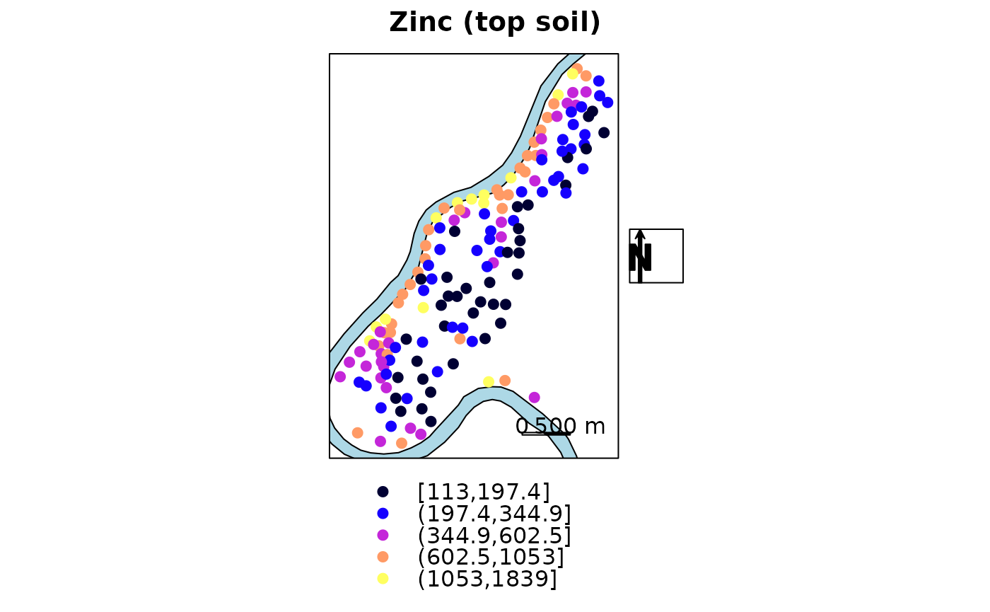
The same plot; north arrow now inside panel, with custom panel function instead of sp.layout
spplot(meuse, "zinc", panel = function(x, y, ...) {
        sp.polygons(meuse.riv, fill = "lightblue")
        SpatialPolygonsRescale(layout.scale.bar(), offset = c(179900,329600),
            scale = 500, fill=c("transparent","black"))
        sp.text(c(179900,329700), "0")
        sp.text(c(180400,329700), "500 m")
        SpatialPolygonsRescale(layout.north.arrow(),
            offset = c(178750,332500), scale = 400)
        panel.pointsplot(x, y, ...)
    },
    do.log = TRUE, cuts = 7,
    key.space = list(x = 0.1, y = 0.93, corner = c(0,1)),
    main = "Top soil zinc concentration (ppm)")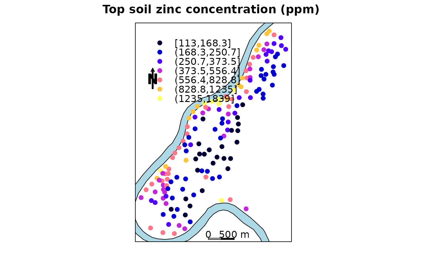
A multi-panel plot, scales + north arrow only in last plot: using the
which argument in a layout component (if
which=4 was set as list component of sp.layout, the river
would as well be drawn only in that (last) panel)
rv = list("sp.polygons", meuse.riv, fill = "lightblue")
scale = list("SpatialPolygonsRescale", layout.scale.bar(),
    offset = c(180500,329800), scale = 500, fill=c("transparent","black"), which = 4)
text1 = list("sp.text", c(180500,329900), "0", cex = .5, which = 4)
text2 = list("sp.text", c(181000,329900), "500 m", cex = .5, which = 4)
arrow = list("SpatialPolygonsRescale", layout.north.arrow(),
    offset = c(181300,329800),
    scale = 400, which = 4)
cuts = c(.2,.5,1,2,5,10,20,50,100,200,500,1000,2000)
spplot(meuse, c("cadmium", "copper", "lead", "zinc"), do.log = TRUE,
    key.space = "right", as.table = TRUE,
    sp.layout=list(rv, scale, text1, text2, arrow), # note that rv is up front!
    main = "Heavy metals (top soil), ppm", cex = .7, cuts = cuts)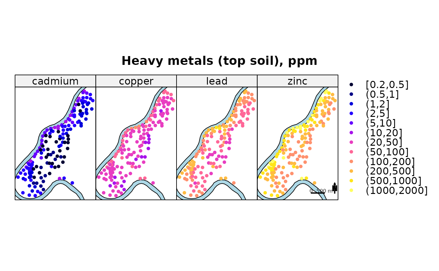
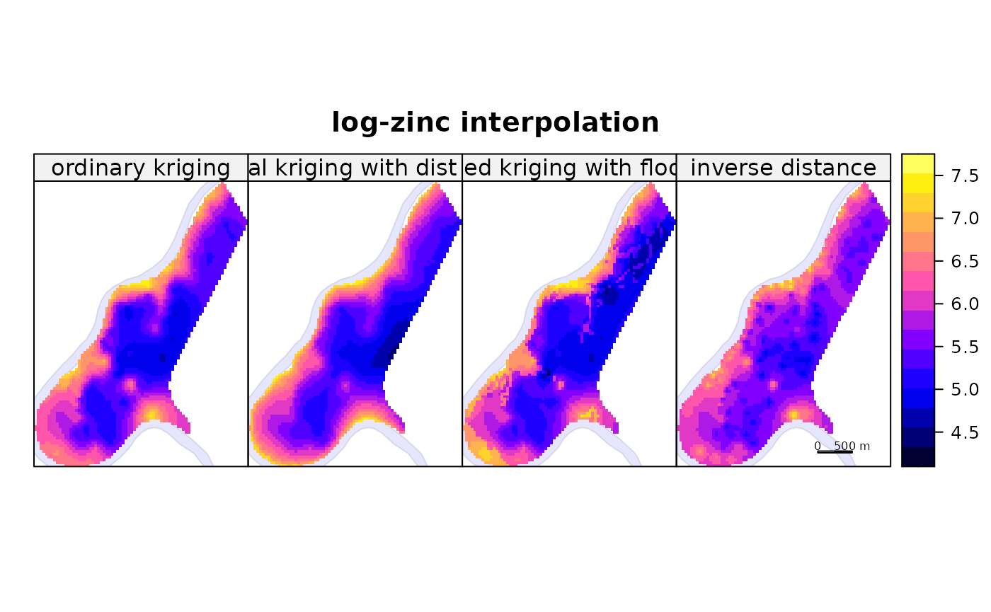
Comparing four kriging varieties in a multi-panel plot with shared scale:
rv = list("sp.polygons", meuse.riv, fill = "blue", alpha = 0.1)
pts = list("sp.points", meuse, pch = 3, col = "grey", alpha = .5)
text1 = list("sp.text", c(180500,329900), "0", cex = .5, which = 4)
text2 = list("sp.text", c(181000,329900), "500 m", cex = .5, which = 4)
scale = list("SpatialPolygonsRescale", layout.scale.bar(),
    offset = c(180500,329800), scale = 500, fill=c("transparent","black"), which = 4)
library(gstat)
v.ok = variogram(log(zinc)~1, meuse)
ok.model = fit.variogram(v.ok, vgm(1, "Exp", 500, 1))
# plot(v.ok, ok.model, main = "ordinary kriging")
v.uk = variogram(log(zinc)~sqrt(dist), meuse)
uk.model = fit.variogram(v.uk, vgm(1, "Exp", 300, 1))
# plot(v.uk, uk.model, main = "universal kriging")
meuse[["ff"]] = factor(meuse[["ffreq"]])
meuse.grid[["ff"]] = factor(meuse.grid[["ffreq"]])
v.sk = variogram(log(zinc)~ff, meuse)
sk.model = fit.variogram(v.sk, vgm(1, "Exp", 300, 1))
# plot(v.sk, sk.model, main = "stratified kriging")
zn.ok = krige(log(zinc)~1,          meuse, meuse.grid, model = ok.model, debug.level = 0)
zn.uk = krige(log(zinc)~sqrt(dist), meuse, meuse.grid, model = uk.model, debug.level = 0)
zn.sk = krige(log(zinc)~ff,         meuse, meuse.grid, model = sk.model, debug.level = 0)
zn.id = krige(log(zinc)~1,          meuse, meuse.grid, debug.level = 0)

zn = zn.ok
zn[["a"]] = zn.ok[["var1.pred"]]
zn[["b"]] = zn.uk[["var1.pred"]]
zn[["c"]] = zn.sk[["var1.pred"]]
zn[["d"]] = zn.id[["var1.pred"]]
spplot(zn, c("a", "b", "c", "d"),
    names.attr = c("ordinary kriging", "universal kriging with dist to river",
        "stratified kriging with flood freq", "inverse distance"),
    as.table = TRUE, main = "log-zinc interpolation",
    sp.layout = list(rv, scale, text1, text2)
)
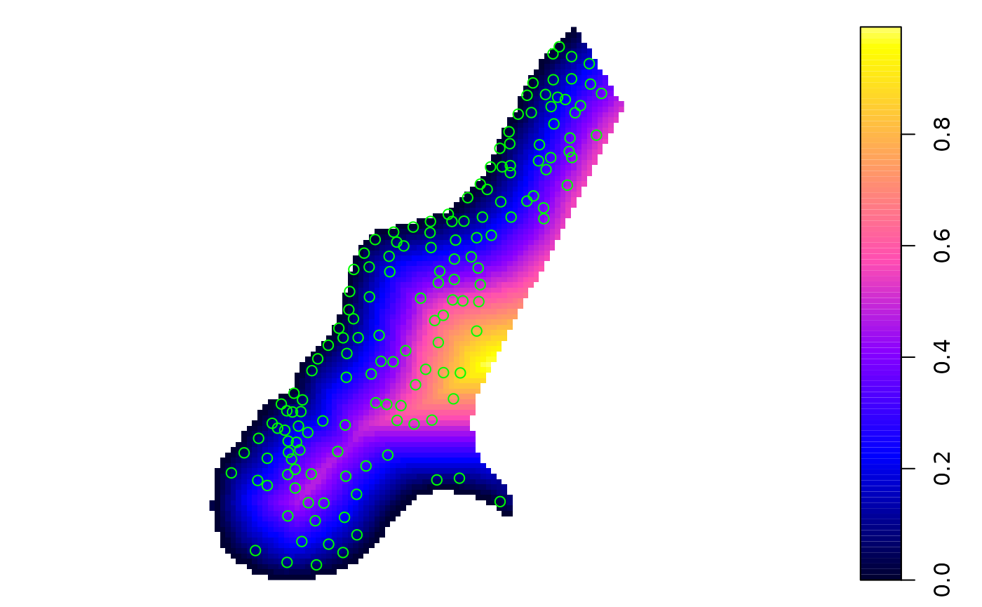
Reuse these results; universal kriging standard errors; grid plot with point locations and polygon (river):
rv = list("sp.polygons", meuse.riv, fill = "blue", alpha = 0.1)
pts = list("sp.points", meuse, pch = 3, col = "grey", alpha = .7)
spplot(zn.uk, "var1.pred",
    sp.layout = list(rv, scale, text1, text2, pts),
    main = "log(zinc); universal kriging using sqrt(dist to Meuse)")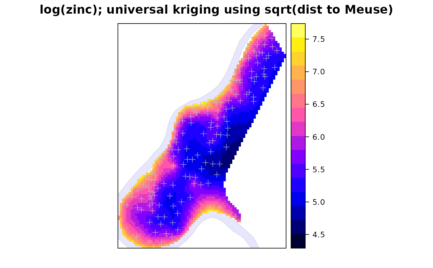
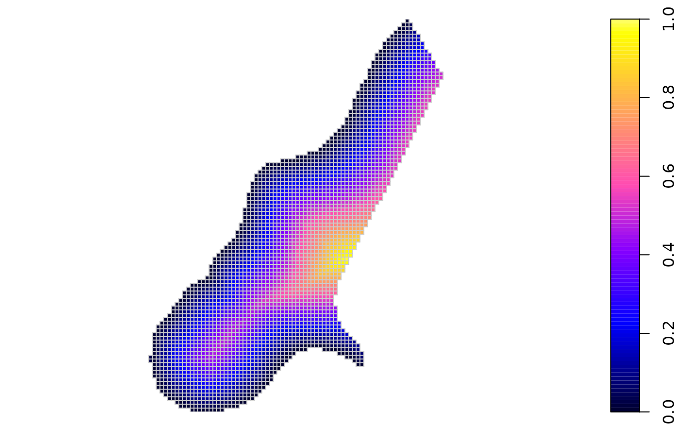
zn.uk[["se"]] = sqrt(zn.uk[["var1.var"]])
spplot(zn.uk, "se", sp.layout = list(rv, pts),
    main = "log(zinc); universal kriging standard errors")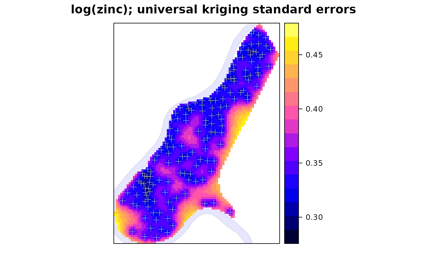
arrow = list("SpatialPolygonsRescale", layout.north.arrow(),
    offset = c(-76,34), scale = 0.5, which = 2)
spplot(nc, c("SID74", "SID79"), names.attr = c("1974","1979"),
    colorkey=list(space="bottom"), scales = list(draw = TRUE),
    main = "SIDS (sudden infant death syndrome) in North Carolina",
    sp.layout = list(arrow), as.table = TRUE)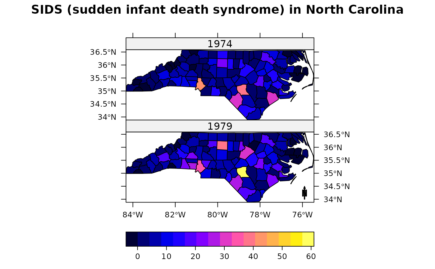
arrow = list("SpatialPolygonsRescale", layout.north.arrow(),
    offset = c(-76,34), scale = 0.5, which = 2)
#scale = list("SpatialPolygonsRescale", layout.scale.bar(),
#   offset = c(-77.5,34), scale = 1, fill=c("transparent","black"), which = 2)
#text1 = list("sp.text", c(-77.5,34.15), "0", which = 2)
#text2 = list("sp.text", c(-76.5,34.15), "1 degree", which = 2)
# create a fake lines data set:
## multi-panel plot with coloured lines: North Carolina SIDS
spplot(nc, c("SID74","SID79"), names.attr = c("1974","1979"),
    colorkey=list(space="bottom"),
    main = "SIDS (sudden infant death syndrome) in North Carolina",
    sp.layout = arrow, as.table = TRUE)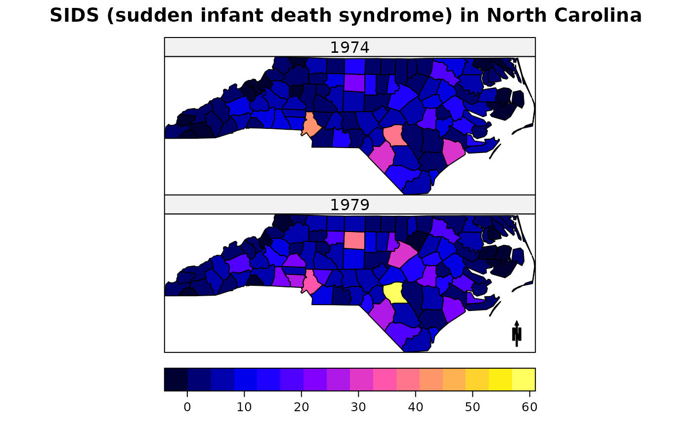
Bubble plots for cadmium and zinc:
b1 = bubble(meuse, "cadmium", maxsize = 1.5, main = "cadmium concentrations (ppm)",
    key.entries = 2^(-1:4))
b2 = bubble(meuse, "zinc", maxsize = 1.5, main = "zinc concentrations (ppm)",
    key.entries =  100 * 2^(0:4))
print(b1, split = c(1,1,2,1), more = TRUE)
print(b2, split = c(2,1,2,1), more = FALSE)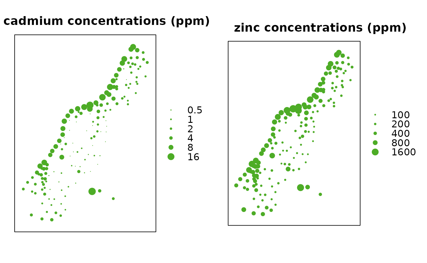
Factor variables using spplot:
# create two dummy factor variables, with equal labels:
set.seed(31)
nc$f = factor(sample(1:5, 100,replace = TRUE),labels=letters[1:5])
nc$g = factor(sample(1:5, 100,replace = TRUE),labels=letters[1:5])
library(RColorBrewer)
## Two (dummy) factor variables shown with qualitative colour ramp; degrees in axes
spplot(nc, c("f","g"), col.regions=brewer.pal(5, "Set3"), scales=list(draw = TRUE))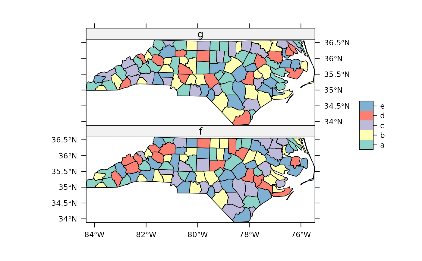
Interactive maps: leaflet, mapview
R packages leaflet and mapview provide interactive, browser-based maps building upon the leaflet javascript library. Example with points, grid and polygons follow:
Mapview also allows grids of view that are synced
m1 <- mapview(meuse, zcol = "soil", burst = TRUE, legend = TRUE)
m2 <- mapview(meuse, zcol = "lead", legend = TRUE)
m3 <- mapview(meuse, zcol = "landuse", map.types = "Esri.WorldImagery", legend = TRUE)
m4 <- mapview(meuse, zcol = "dist.m", legend = TRUE)
sync(m1, m2, m3, m4) # 4 panels synchronised
# latticeView(m1, m2, m3, m4) # 4 panels
more examples are found here.
SessionInfo
## R version 4.4.0 (2024-04-24)
## Platform: x86_64-pc-linux-gnu
## Running under: Ubuntu 22.04.4 LTS
##
## Matrix products: default
## BLAS:   /usr/lib/x86_64-linux-gnu/openblas-pthread/libblas.so.3
## LAPACK: /usr/lib/x86_64-linux-gnu/openblas-pthread/libopenblasp-r0.3.20.so;  LAPACK version 3.10.0
##
## locale:
##  [1] LC_CTYPE=C.UTF-8       LC_NUMERIC=C           LC_TIME=C.UTF-8
##  [4] LC_COLLATE=C.UTF-8     LC_MONETARY=C.UTF-8    LC_MESSAGES=C.UTF-8
##  [7] LC_PAPER=C.UTF-8       LC_NAME=C              LC_ADDRESS=C
## [10] LC_TELEPHONE=C         LC_MEASUREMENT=C.UTF-8 LC_IDENTIFICATION=C
##
## time zone: UTC
## tzcode source: system (glibc)
##
## attached base packages:
## [1] stats     graphics  grDevices utils     datasets  methods   base
##
## other attached packages:
## [1] mapview_2.11.2     RColorBrewer_1.1-3 gstat_2.1-1        maps_3.4.2
## [5] sf_1.0-16          sp_2.1-4
##
## loaded via a namespace (and not attached):
##  [1] xfun_0.43               bslib_0.7.0             raster_3.6-26
##  [4] htmlwidgets_1.6.4       lattice_0.22-6          leaflet.providers_2.0.0
##  [7] vctrs_0.6.5             tools_4.4.0             crosstalk_1.2.1
## [10] stats4_4.4.0            proxy_0.4-27            spacetime_1.3-1
## [13] highr_0.10              xts_0.13.2              KernSmooth_2.23-22
## [16] satellite_1.0.5         desc_1.4.3              leaflet_2.2.2
## [19] uuid_1.2-0              lifecycle_1.0.4         farver_2.1.1
## [22] compiler_4.4.0          FNN_1.1.4               textshaping_0.3.7
## [25] munsell_0.5.1           terra_1.7-71            codetools_0.2-20
## [28] htmltools_0.5.8.1       class_7.3-22            sass_0.4.9
## [31] yaml_2.3.8              pkgdown_2.0.9           jquerylib_0.1.4
## [34] classInt_0.4-10         cachem_1.0.8            brew_1.0-10
## [37] digest_0.6.35           purrr_1.0.2             fastmap_1.1.1
## [40] grid_4.4.0              colorspace_2.1-0        cli_3.6.2
## [43] magrittr_2.0.3          base64enc_0.1-3         leafem_0.2.3
## [46] e1071_1.7-14            scales_1.3.0            rmarkdown_2.26
## [49] ragg_1.3.0              zoo_1.8-12              png_0.1-8
## [52] memoise_2.0.1           evaluate_0.23           knitr_1.46
## [55] rlang_1.1.3             Rcpp_1.0.12             leafpop_0.1.0
## [58] glue_1.7.0              DBI_1.2.2               svglite_2.1.3
## [61] jsonlite_1.8.8          R6_2.5.1                systemfonts_1.0.6
## [64] fs_1.6.4                intervals_0.15.4        units_0.8-5